Real-Time Recurrent Learning: Training Dynamics
Learning online the parameters of a Recurrent Neural Network (RNN) holds the promise of offering better sample complexity when compared to offline algorithms such as Backpropagation Through Time. We benefit from the stable parametrization of the Linear Recurrent Unit, to study the training dynamics of the Real Time Recurrent Learning (RTRL) algorithm in the class of linear RNNs. We show empirically and justify theoretically that RTRL benefits from highly stochastic online updates. From the insights we develop in the linear setting, we then study it’s implications in highly sparse Continuous Time Recurrent Neural Networks were we observe similar results. Overall, our findings allow us to offer a possible explanation for the phenomena observed by other researchers when training highly sparse RNNs with RTRL.
1 Online vs Offline
Let’s start by introducing the notation we’ll use throughout this post. We define the transition function as , where denotes a finite dimensional vector space where the parameters live, denotes the same for the hidden states and as well for the inputs to the RNN. A single sequence of inputs will be defined as where denotes the end of the sequence. For when needed we define and to further declutter notation given a fixed input we define . For a fixed parameter , given an initial condition , the sequence of hidden states produced by the network can be recursively defined as:
Under this formalism an RNN can be considered a non-autonomous discrete dynamical system.
In what follows we focus on gradient-based learning where the objective is to minimize at each time step , a cost function that measures the network's performance on a given task, as a function of the parameters . Note that can be unbounded, but in this post we focus on the case where . This allows us to define a cumulative loss function:
that will measure the overall performance of the network.
In the Sparse Jacobians post, we introduced two different algorithms to compute the gradient . Backpropagation Through Time (BPTT) and Real Time Recurrent Learning (RTRL). Both algorithms are equivalent, in the sense that they compute the same gradient , the difference however relies on how this gradient is computed. BPTT computes the cumulative loss gradient in two passes, a first forward pass where the inputs are processed, and a second backward pass where the gradients are computed. In contrast RTRL allows for comuting both in just a single pass, however this comes at a significant computational and memory cost as explained in the Sparse Jacobians post. More specifically RTRL computes each explicitly as the network runs, whereas BPTT will only compute them implicitly. To better illustrate this difference we can derive the gradient equations for both methods:
after the exchange of summations in BPTT we are not computing by adding each , but rather different terms. RTRL computes by adding each explicitly as we process the inputs.
Being able to obtain the gradient of the instantenous loss as we process the inputs is the core feature of RTRL. It allows the update of the parameters in an online fashion, without having to neither accumulate the gradients nor wait until the sequence has been fully processed. This is what we refer as the online training setting, where numerous updates of the parameters are performed as we process the inputs, in contrast to the offline training setting in which only one update of the parameters its performed at the end. Throughout the rest of this post to remove unnecessary wording we will refer to RTRL with online updates as the online algorithm, and to BPTT as the offline algorithm. A single online update of the parameters while processing an input will be refered as an in-sequence update, to better emphasize its nature.
To make the difference more clear between both training settings, we can make explicit the dependence of the parameters on . In the offline setting we are not performing any update as we run the network, therefore we have for , whereas in the online setting in general we have for . We remark that this change of parameters as the network runs only happens while training, and when doing inference on a new input sequence the parameters are fixed for both methods1.
Online updates of the network parameters can exhibit different training dynamics when compared to their counterpart. This difference arises by noting that while in the offline setting:
in online setting we have:
therefore, except for the first time step, in the online setting we are no longer computing the real Jacobian but a biased one, that will a priori better reflect the influence of the most recently used parameters in comparison to the initial ones . If we use gradient descent, this bias will imply that we are no longer following the precise negative gradient direction. The difference at each step is nevertheless , so one can mitigate this bias by reducing the learning rate. The bias of the when using online updates, was indeed noted by the original authors of RTRL [1]:
While the resulting algorithm is no longer guaranteed to follow the gradient of total error, the practical differences are often slight, with the two versions becoming more nearly identical as the learning rate is made smaller.
By making small we are potentially aligning more closely to BPTT training dynamics. Even in this small learning rate regime formally analyzing the online algorithm becomes substantially challenging since standard stochastic gradient descent theory does not apply directly, and to this date we could only find one work where they proved local converge of RTRL when the network parameters start within a radius close enough to a local minima [2].
Local converge itself will not really tell us much about the qualitative differences on the training dynamics when the network has just been initialized with random parameters. It is the purpose of this post to try elucidate the qualitative differences, if any, that arise when using RTRL with online updates in comparison to BPTT. To the best of our knowledge no prior work has been done in this regard, and even though numerous studies have been done in either improving, or analyzing the performance of RTRL in different scenarios, as well as reducing its computational cost, we could not find any prior work in trying to uncover the qualitative differences that could potentially arise.
2 Teacher Student Analysis
2.1 Online EVGP
As argued in [3] if there is any hope of understanding Recurrent Neural Networks we first need to understand them in the special case where we remove the non-linearities. Albeit in principle this simplifies the analysis, removing the non-linearities however makes the online algorithm more prone to the exploding-vanishing gradient problem [4], when compared to the offline one. To see this, lets first define , , and . Equation 3 can then be rewritten as:
unrolling the recurrence and starting with , we can see that:
In the class of linear RNNs2 and when using the offline algorithm the state-transition Jacobian becomes constant , therefore by computing we are also computing . This becomes an issue if the spectral radius3 is strictly bigger than since the gradients are computed using and therefore as grows we enter the exploding gradient regime. This can be partially mitigated by ensuring that at initilization the randomly sampled satisfies the condition , however an update of the weights could easily break this inequality.
Even though this is a big concern in both algorithms, note that in the online setting the state-transition Jacobian is not constant anymore, since we are updating at every time step . With no non-linearity regulating the matrix products in , a single bad in-sequence update could already set the RNN in the unstable regime. Therefore even in the linear setting, studying the dynamics of the online algorithm becomes more difficult. Recall that reducing the learning rate to smaller values in order to control the perturbation of an in-sequence update is ideally not what we are aiming for, since as mentioned before this will lead to training dynamics similar to BPPT. To further make progress in our study, we are going to take advantage of the Linear Recurrent Unit, recently introduced by [5].
2.2 Linear Recurrent Unit
Let be the connectivity matrix of a linear RNN, the input matrix, and the readout matrix. Given , and a sequence the output is computed as:
this in fact is equivalent to computing the convolution:
note that diagonalizable matrices are dense in [6], therefore under a small perturbation of we can decompose it as , where , and is an invertible matrix. Left multiplying equation 5 by on both sides, and letting , , we obtain:
If the purpose of our study is to first understand the training dynamics of RTRL in the class of linear RNNs, we might as well train linear RNNs where instead of learning , we learn 4 and work with complex matrices. Expressiveness will not be lost in this parametrization, but it still does not ensure stable training dynamics and the EVGP remains a concern in both online and offline training settings.
Recently [5] took the previous approach one step further, and propose parametrizing the elements of as:
where it is the vectors and that will be learned during training. It is easy to see that under this parametrization starting with for all guarantees at initialization. However post-update stability cannot be guaranteed since a can become negative. To address this, they introduced an additional positive non-linearity leaving the final parametrization as:
and now stability is ensured post-update. For learning long-range sequences where , the authors still noted a explosion in the forward pass. To see why5, assume a one dimensional network , and let . Then under white-noise input we can see that:
therefore as the forward pass explodes since the contribution from takes longer to decay. In order to address this issue they propose to normalize by an element-wise factor defined at initialization as .
Given the preceding normalization and the exponential parametrization of (7) the Linear Recurrent Unit (LRU) is formally defined by [5] as:
where . The LRU plays a significant role for our next studies as in-sequence updates will no longer break the stability of the linear RNNs. Furthermore as shown by [7], the diagonal nature of the connectivity matrix in the LRU allows for drastically reducing the computational and memory requirements induced by RTRL. This is due to the fact that complex neurons in the LRU do not affect each other and therefore tracking the sensitivities requires only storage, while updating the Jacobian gets reduced from a matrix multiplication to a dot product. For more details about the properties of the LRU and its online training algorithm the reader is encouraged to check the excellent work done by [5] and [7].
Having introduced the LRU and its benefits when used in combination with the RTRL algorithm, in the next section we will start studying its dynamics empirically in a teacher-student setting.
2.3 Sample Complexity Study
Our investigation begins with the question: Does the substantially higher update frequency of RTRL compared to BPTT provide any benefits in a Linear System Identification (LSI) task? Specifically, we aim to determine whether it results in improved performance or faster convergence.
Following [8], we will work under a teacher-student setting where the teacher is formally defined as:
with , drawn i.i.d. from , , , and . The difficulty of the task its determined by the spectral radius of , since given an input its contribution to is modulated by as can be seen from equation 6. Thus bigger values of will force the student to remember inputs from further back in time. Since this is a parameter we want to control in our experiments, after sampling , we complex diagonalize it6, and then we apply the following transformation [8] to its spectrum:
note that this transformation ensures that . In case contained complex eigenvalues they must come in conjugate pairs. By using in the transformation and noting that , the resulting matrix after the transformation is also real.
Controling and in the teacher is not enough for our purposes as we also need to control the spectrum of the student. The student will be a LRU, where its spectrum is controled by sampling using lemma 3.2 from [5]:
Let be independent uniform random variables on the interval . Let . Compute , where and . Then is uniformly distributed on the ring in between circles of radii and .
For the experiments the hidden size of the teacher is fixed to 10 and for the student 64. We will gradually increase and for the student and the teacher respectively. We choose a sequence size of to ensure that the input sequence is longer than the characteristic timescale we want to learn7. For every value , we train the student LRU with BPTT and RTRL under the same conditions with the same budget of samples, which varies from . We work under the purest version of SGD with batch size . The loss is the mean squared error over the prediction and the target sequence. To be fair with both algorithms and since gradient descent optimization is highly dependent on the learning rate, we sweep over 15 learning rates starting from and decreasing logarithmically. For the optimization algorithm we use Adam [9] with its default hyperparameters in combination with cosine annealing without warm restarts8. When the best evaluation loss is found at one of the extremes of the allocated learning rates, we manually finetune it until the best learning rate does not live in the extremes. We repeat everything for different seeds. The grid search is done using Ray Tune [10], and we use the framework introduced in the Sparse Jacobians post for implementing RTRL, where we conducted unit tests in all the optimization algorithms to ensure their correctness. Details of all the hyperparameters that we sweep over can be found in table 1.
Intuitively to correctly explore the parameter space for learning long-range dependencies, we want the to not be biased. This is ensured in BPPT, as there are no in-sequence updates. However for RTRL this term does not actually reflect the influence of the parameters at the beginning of the sequence. Since has had an influence in and in turn influences as well, if the loss at time step is highly dependent in the state of , we should take into account the that leads to as well.
By allowing online updates we are not really tracking the real influence over all time steps. For tasks with short-time scale as measured by the spectral radius of the teacher, we should expect that the significantly higher number of updates of RTRL help converging faster towards a smaller loss. This advantage however should be lost as we give more sample budget both BPTT and RTRL, and the spectral radius of the teacher increases as well.
Results of the empirical sample complexity experiment for LSI can be seen in figure 1. The results align with our intuition as the performance of RTRL outperforms BPPT only on small values of and when the budget of samples is small. Eventually the differences vanish and BPTT catches up in performance. For bigger values of , RTRL does not present any advantage and when the budget is increased towards performs an order of magnitude worse than BPTT.
Grid Search
| Algorithms | {RTRL, BPTT} |
|---|---|
| Samples | |
| Seeds | |
| Teacher | 10 |
| Student | 64 |
| Batch Size | 1 |
| 1 | |
| Scheduler | Cosine Annealing (No warm restarts) |
| 0.9 | |
| 0.99 |
Table 1: Experimental details of the grid search performed for the empirical sample complexity study.
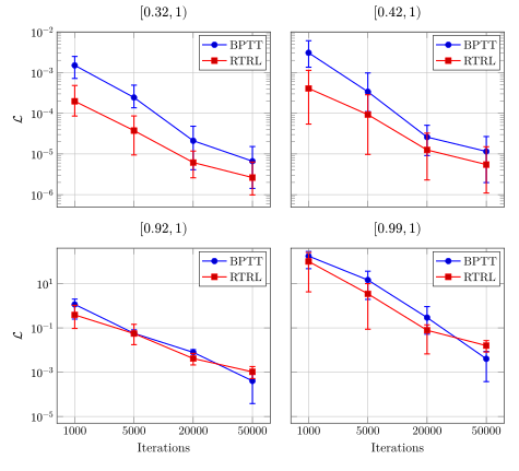
Figure 1: Sample complexity study for different values of . We report the mean over all the seeds, where the error bars denote the min and max over the seeds. Both BPTT and RTRL are in their best performing setting, found with grid search.
3 Benefits of Noisy In-Sequence Updates
Recall that in the previous experiment we used Adam with its default hyperparameters as our optimizer. Lets take a closer look at the update function defined by Adam9:
Adam defines three10 hyperparameters , and that are left for the experimenter to tune. Intuitively controls the exponential moving average of the gradients, since as greater smoothing is performing and more weight is given to the average gradient . One will expect that for learning a long-range task, if we are performing in-sequence updates, we want to give more importance to the average gradient , the intuition for this is that since in the online setting the parameters now define a in-sequence trajectory , the update directions from the instantaneous loss gradients do not necessarily need to be aligned11. This leads the trajectory to fluctuate significantly, which we control using with Adam. The interpretation that controls these fluctuations of the gradients, can be easily checked by tracking the updates 12 given by Adam to the eigenvalues, as we do in Figure 2.
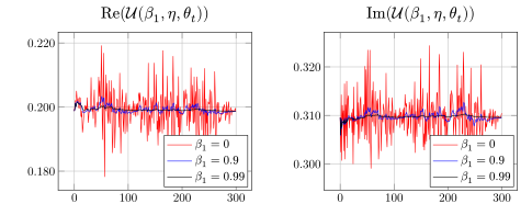
Figure 2: Toy example to confirm our intuition regarding the role of the in Adam for in-sequence updates. One dimensional teacher in , one dimensional student dimensional student in . One single iteration of RTRL over an input sequence.
Whether reducing this fluctuations is beneficial for RTRL, as we presuppose, is what we discuss next.
Contrary to our intuition the closer the better RTRL performs, even in the harder task of our previous experiment where . In figure 3, we can see a sweep over different values of , where for each , we follow a similar grid search procedure as in the previous study, ensuring that for every we find the best configuration, ensuring a fair comparison. The best mean performance its achieved with i.e no smoothing at all over the in-sequence gradients, and even more surprising, it is achieved with the maximum initial learning rate when compared to best performant learning rates in the other scenarios.
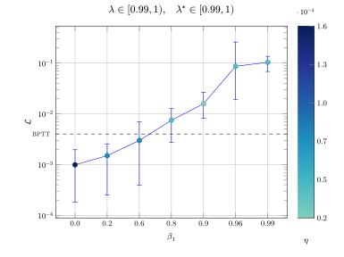
Figure 3: Performance of Adam in the LSI task for different values of . The colorbar reflects the value of the initial learning rate . Cosine Annealing is applied for every run. Mean of 4 different seeds, errors bars indicating the min and max evaluation loss.
In order to get more insights we start by analyzing the backward sensitivity of the system, which we define as:
where the norm is the spectral norm i.e the largest singular value. Intuitively this term measures how sensitive the final hidden state is to a perturbation of a hidden state in a distant past . For tasks with long-range dependencies we want this term to increase during training in case it is small at time steps the task cares about.
Note that in the LRU, the state-transition Jacobian is constant , and because the spectral norm of a diagonal matrix its equal to its spectral radius we have that . So function 11 its completely characterized by the spectral radius of , which allows us to study it with just a single scalar. Therefore we track the eigenvalue after every iteration of both RTRL and BPTT, as well as tracking the eigenvalue and then mean of . We do this in a setup where the student starts with a spectrum in , so that we recover Glorot initialization [11]. The teacher will be set to the hardest difficulty where , in addition to . For both algorithms we follow the same grid search procedure as in the previous study in order to compare them in their best performing settings. Since we want to better understand the observation from figure 3, in RTRL we check for and , whereas in BPTT we only check for . Note that in the class of Liner RNNs, as mentioned before, the state-transition Jacobian is constant13 and is equal to the connectivity matrix, therefore we should expect in both settings that the spectral radius of increases towards higher values, closer to where the spectral radius of the teacher is. Otherwise they could not learn the long-range dependencies.
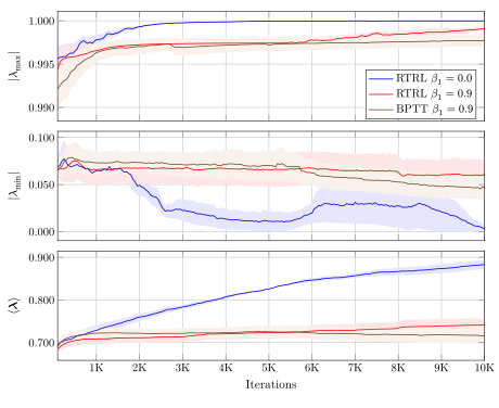
Figure 4: Evolution of the norm of max, min and average eigenvalue during the first 10K iterations. Student initialized in . Teacher initialized with in . Shaded areas indicate the standard error of the mean over the different seeds.
In figure 4 we can see the evolution of the quantities just described. From the plots we note three qualitative differences when considering noisy in-sequence updates () in comparison to BPTT and smoother in-sequence updates () in RTRL:
-
The spectral radius converges faster towards its theoretical limit14.
-
The norm of the minimum eigenvalue converges faster towards 0.
-
Overall the norm of the eigenvalues of the state-transition Jacobian tend to converge faster towards higher values.
in order to better comprenhend this empirical observations, in the next subsection we will argue for a simple toy model that we believe explains the previous qualitative differences.
3.1 RTRL Toy Model
To understand the qualitative phenomena of the previous study we start by recalling the LRU parametrization15:
where and . Since the quantity we are interested is the norm of , to simplify the analysis we set as it does not contribute16 to the norm. Therefore the parametrization we study is left as:
and the in-sequence update equations17 when performing gradient descent follow:
Define , and note that , hereby equation 13 becomes:
we can treat 15 as a non-autonomous discrete dynamical system, since will be varying at each time step . Even though an oversimplification, is still worth assuming constant , so that we can treat 15 as an autonomous dynamical system, where the analysis becomes easier. In the one-dimensional setting the direction of is either a positive one or negative , so assuming , we can plot the dynamics of the system in a Cobweb diagram (Figure 5) together with the LRU parametrization. From the plots it is clear that:
Of course during optimization neither will be constant nor . The term will be regulated by the learning rate , and the directions will differ during the in-sequence updates. In RTRL fluctuates significantly during the forward pass (Figure 2), and this fluctuation can be controlled by when using Adam.
Assuming, as previously argued, that fluctuates significantly, let's replace by a random variable . The fluctuation is now governed by . Consider a Markovian random walk in . With sufficient iterations, the larger the the quicker the random walk reaches its first-passage time for a given threshold. Recalling that in RTRL we perform additional updates to compared to BPTT, the previous analysis suggests that under in-sequence updates, convergence towards either 0 or 1 occurs more rapidly in the LRU, even if these updates exhibit considerable fluctuation. In fact larger fluctuations, as in the random walk, imply earlier first-passage times over values of that result in closer values of to the two poles. We can see now that as , the effective increases, leading to a faster increase in the spectral radius while training, thereby enhancing performance in the harder task where , which is what we see in figure 4.
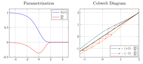
Figure 5: Left: Parametrization of the LRU for real eigenvalues. Right: Cobweb Diagram assuming constant backpropagated errors, or
In figure 6 we confirm our analysis, where we sample a white noise sequence from to play the role of and we track the evolution of , where , for different values of . As we can appreciate from the figure, the largest value of results in faster convergence towards the two poles, 0 and 1, but eventually for every value of convergence to the poles should occur given enough iterations. We repeat the analysis for white noise sequences, each of them of length , and in figure 6 we show their distribution at different time steps, for different values of . The higher density around 0 in the histogram at 10K can be explained by noting that:
which implies that converge happens in fewer iterations towards 0 than towards 1, biasing the distribution in this simplified RTRL toy model for the LRU.
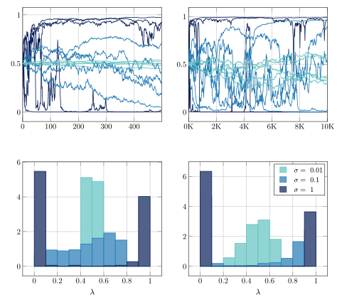
Figure 6: Top: Sampled trajectories of the toy RTRL model, for different standard deviations for steps.Bottom: Distribution at of sampled trajectories for different standard deviations
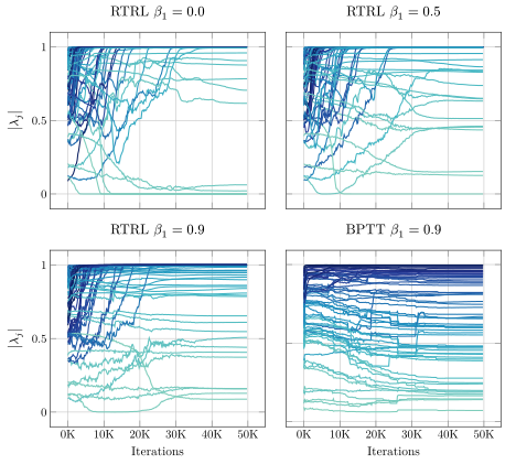
Figure 7: Trajectories of the during training in RTRL for different values of and in BPTT. Coloring reflects the order of , darker being the highest, lighter being the lowest. Only one seed is showed for easier visualization
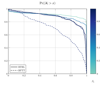
Figure 8: after 50K Iterations of training. Computed over 4 different seeds for different values of and for BPTT.
From the previous analysis we can already start to understand the qualitative differences we observed in the LSI study between the different scenarios and BPTT. If the of the LRU should show convergence towards a bimodal distribution in 0 and 1, which in turn will increase the spectral radius. This is what we indeed observe in figure 7, when we track the trajectories of the during training of the LSI task. Only one seed is displayed for making the visualization easier, nevertheless to strengthen our hypothesis about the qualitative differences between RTRL and BPTT, in figure 8 we plot the complementary cumulative distribution function 18 (CCDF) at the end of training, now computed among the different seeds for both RTRL and BPTT.
Note that the displayed in figure 8 is computed at the last iteration of training, nevertheless given the big gap between BPTT in RTRL it suggests the following. For sufficiently big , there exists a threshold such that for all :
where with we denote BPTT and with we denote RTRL. We cannot offer a proof for this, but nevertheless, we give support for this claim in figure 9, where we show CCDF for both methods while training from the first iteration until iteration 1000, the upper bound on 1 its given by the stable parametrization of the LRU. How small can this be, we believe will become relevant when we study non-linear RNN's in the next section.
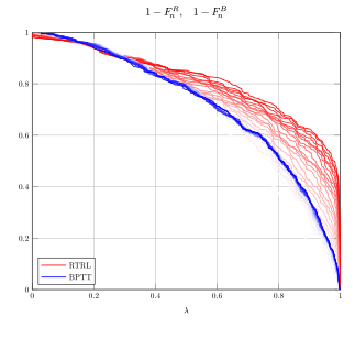
Figure 9: In Red: for . In Blue: for . and . Runs over 4 seeds. Lighter color indicates earlier iterations, darker color indicates iterations at the end.
Interpreting as wast partly motivated by figure 2, where we verified, albeit in a simplistic setting, that the updates provided by Adam i.e , were highly stochastic in nature. The cautious reader must have noted that our definition of in the toy model, doest not equate exactly to our LSI experiments are being performed. To see why note that when using Adam, the actual update equations for follow therefore:
to further strength our observations and justify our interpretation of we need to decompose into the two terms, and so that:
which matches the same equation as in 15, note that in the LRU is a vector in and as well, therefore to solve for , we could right multiply both sides by the inverse matrix . The inverse is guaranteed to exist since the matrix is diagonal19. If our interpretation of RTRL and the influence of is a valid one, then we must see as well that when computing the element-wise (using as observations all the time steps during an input sequence given at iteration ) 20, for different values of the variances must satisfy21:
Recall that is a vector with elements in therefore we use the following definition of variance for a complex random variable:
In figure 10 we can see these values computed using 4 different seeds where we used the same initial learning rate . Note that they closely match our interpretation of .
Overall the previous experiments further validate the use of our toy model for RTRL, when trying to study its dynamics. Though it may sound simple, to the best of our knowledge we have not seen any study in the literature following our approach. This might partially be because of timing, since the LRU which is a key component in our study has only been introduced recently. We conclude this section by reminding the reader that we started studying RTRL in class of linear RNNs, with the hope of giving us a better understanding of its training dynamics in the non-linear setting. In the next section we start to study RTRL in non-linear RNNs.
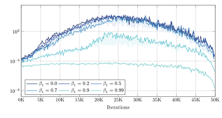
Figure 10: Mean of the vector during training for different values of .
4 Implications In Sparse Networks
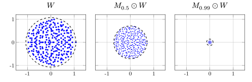
Figure 11: Distribution of the eigenvalues for a random matrix with i.i.d entries from , when applying masks of different levels of sparsity.
Recently [12] showed the advantage of imposing sparsity in the parameters of the network by proposing a biased approximation to which reduces the memory and computational complexity of RTRL, as explained in the Sparse Jacobians post. Their experiments conclude that training highly sparse RNNs (GRU and LSTM) with RTRL outperforms BPTT when learning a curricular copy task. Studying RTRL in RNNs with gated mechanisms to understand this phenomena. Is out of the scope of this thesis and left for future work, here instead we focus on Continuous Time Recurrent Neural Networks (CTRNN), using some of the insights derived from the previous section in Linear RNNs.
Following [13] the class of CTRNN considered here are derived from the discretization of the following continuous-time dynamical system:
where , represents the number of hidden units, the number of input channels, , and . The readouts of the network are computed by:
where represents the number of output channels and . Similar to [13] we are interested in the training dynamics of networks where and the dimensions of , and are small. However we depart from their setup by forcing sparsity in the connectivity matrix in an attempt to understand the results from [12]. We do this by sampling a random binary matrix with entries , where will control the amount of sparsity imposed in the connectivity matrix. The transformation to is simply:
The first insight to understand [12] comes from the following fact. Define , if the entries then:
since and , then22 by Bai and Yin [14], we have that:
and by reverse Fatou's Lemma:
which basically tells us that for (as in our setting and the one in [12]), under Glorot initialization of the connectivity matrix , imposing a random mask on the weights to induce sparsity, effectively decreases its spectral radius. This behavior is illustrated in Figure 11. In the regime of linear RNNs, as discussed in the previous section, RTRL should escape this small spectral radius faster than BPTT. As a result, this could potentially enhance performance when the objective is to learn long-range dependencies, which is what [12] observed in their experiments although in highly sparse gated RNN's.
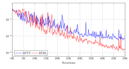
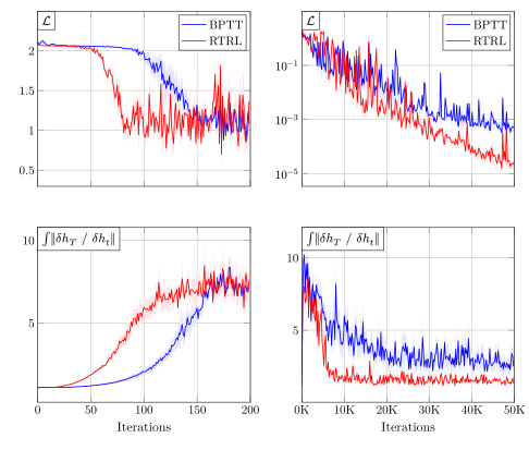
Figure 12: Mean Squared Loss curves RTRL and BPTT in the evaluation distribution. Average over 4 different seeds. Both RTRL and BPTT in their best performing setting after running a comprehensive grid search. Shaded regions represent the standard error of the mean of the quantity of interest.
To test the hypothesis that RTRL outperforms BPTT when training highly sparse CTRNN we will follow a similar approach as in the preceding section were now we substitute the LSI task, with the Romo [15] task. The task is a delayed-discrimination task, where the network is presented with two positive pulses of different amplitudes separated by a delay. Following an additional delay, the network is required to remember which of the two pulses had greater amplitude. We choose this task as it is a simple one to start studying RTRL and we can easily control the specific time steps at which the network has received its inputs and has to start recalling the largest pulse.
As in all of our previous experiments to compare BPTT and RTRL in their best performing settings, we follow a similar grid search as in the sample complexity study. For RTRL we set in light of the previous section and for BPTT we set . The sparsity of the network is imposed by sampling a random binary mask as explained before were we set to 0.98. For the size of the hidden units we choose following [13] and also to obtain the upper bound in 23. For discretizing 20 we choose as . The evaluation loss is the mean squared error over the readouts of the network. The number of iterations for both RTRL and BPTT is set 50K. Similar to the LSI task we set the batch size to 1. In figure 12 we can see the evaluation loss curves for both methods in their best performint setting. Clearly RTRL outperforms BPTT. This partial result strengthen our hypothesis about the advantages of RTRL in highly sparse CTRNNs. In figure 13 we can also see how the spectral radius converges substantially faster to a bigger value in RTRL23. We have run control experiments where after sampling the random sparse connectivity matrix, we scale it so that we start in both algorithms with , and the result in terms of performance were almost the same, with RTRL clearly outperforming BPTT. Therefore there has to be some other qualitative phenomena explaining the gap in performance.
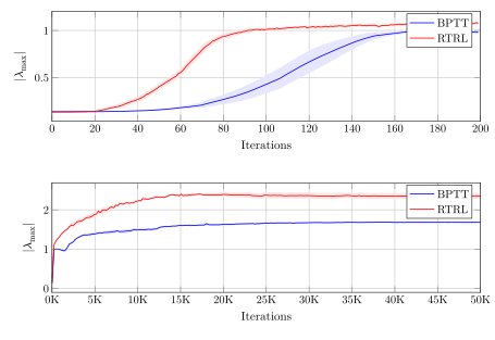
Figure 13: Evolution of the spectral radius . Average over 4 different seeds. Both RTRL and BPTT in their best performing setting after running a comprehensive grid search. Shaded regions represent the standard error of the mean of the quantity of interest. Top: Evolution during the first 200 iterations. Bottom: Evolution for the full training loop.
Note that in the non-linear regime, the spectral radius is not a good indicative anymore of how the network is learning, in the case of the LRU we studied that term since as commented before, the backward sensitivity function can be fully characterized by a single scalar. This is not true in the case of non-linear RNN's. The state-transition Jacobian of CTRNN after discretization is not constant anymore and follows:
In an attempt to understand the difference in performance between both methods we recall the following standard result in the theory of continuous-time dynamical systems. Assume we have an ODE, defined as:
where and represents the hidden states of a non-linear RNN. We can differentiate equation 25 from both sides with respect to and after an exchange of derivatives24 we get the following equation:
note that its closely related to the function 11 we were studying in the previous section, were instead the role of the time variable is inverted. Intuitively measures how sensitive is with respect to a perturbation to the initial condition . Following [16] lets define as well , equation 26, can be rewritten then as an ODE following:
where . Similar to [16] we are going to make the assumption that is constant, although a strong assumption its going to help us understand the qualitative differences of RTRL when compared to BPTT, at least in the Romo task. The strong assumption, thus allows us to get the solution for the ODE at 27:
assuming that is diagonalizable we then get:
where denotes the eigenvalues of . Using the fact that the trace bounds the spectral norm, we have then:
combining this lower bound, with the results from figure 9 (where we showed empirically that early in training of a LRU, RTRL has much higher probability than BPTT of for bigger values of ), we can see that RTRL also early in training will increase the trace in 30 since:
and as grows this term will be dominated by the with highest absolute value, which is precisely what RTRL increases from what we observed in the previous experiments. Therefore RTRL will push the lower bound in 30 to higher values, biasing as well the spectral norm of the forward sensitivity towards higher values when compared to BPTT early in training, which is needed to in order to start learning distant dependencies in a sequence [4]. Note that we have made strong assumptions in the previous derivation, which don't necessarily have to match the real experimental setting. In what follows we study what we have just argued.
In light of the previous experiments and from 23 we hypothesize that RTRL bias Highly Sparse CTRNNs to two regimes during training, the first one, suggested by 30, where the network tries to memorize as much as possible, and then learns to forget the irrelevant inputs for the task at hand. Actually we hypothesize that both BPTT and RTRL use the same strategy since the spectral radius of the network at initialization its quite small, but RTRL will enter the regime of memorizing much faster.
To study this hypothesis we follow a similar approach as in the previous section. As a reminder, we want to analyze:
For every new input sequence this function changes, therefore we are not interested in the absolute magnitudes of 32 within a sequence, we are interested in their relative values within a sequence. For example, we could be interested in comparing the value at a fixed time step but at different iterations of the training algorithm say . At iteration the could be much smaller in norm than at . However that does not indicate that network its less sensitive to a perturbation in at iteration , as it could be that the its the biggest value in norm within its sequence indicating the contrary. Therefore if not normalizing this quantity we cannot compare them in fair manner during training at different iterations. For this reason the actual term we track is the following one. Define for iteration of the algorithm, the quantity we track can be defined then as:
this quantity is bounded in therefore we could also integrate it, and track as well:
so that we can display in a simple way the evolution of the overall backward sensitivity of the algorithms. In figure 14 we can see 33 for a single seed and for only one input sequence at different number of iterations during training, already supporting our intuition about RTRL increasing norm of the backward sensitivity faster early in training. In figure 15 we can see 34, which gives even more support to the hypothesis that RTRL converges faster to a bigger value of 34, and then decreases this term faster as well compared to BPTT. We find interesting that even though their respective evaluation losses follow similar trends at the beginning of training, there exists a qualitative difference hidden in the dynamics of 34.
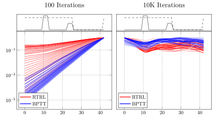
Figure 14: Left: Normalized for the first 100 iterations of the algorithm. Right: Normalized for the first 10000 iterations of the algorithm. Ligher color indicate ealier iterations, darker colors indicate iterations close to the end. Only one sample, and only seed is displayed for easier visualization.
Figure 15: Top Row: Evaluation loss curves. For 200 and 50K Iterations. Bottom Row: Integral of the normalized backward sensitivity for 200 and 50K Iterations. Shaded areas indicate the standard error of the mean for the quantity of interested. Average over 4 different seeds. Both RTRL and BPTT in their best performing settings, found by a comprehensive grid search.
We conclude this short section and the post by remarking that our study although small in nature, offers an possible explanation for the results obtained in [12]. RTRL benefits from highly stochastic in-sequence updates, and it benefits even more when the network is highly sparse, as we showed experimentally and motivated theoretically. We also posit a potential negative consequence: the tendency of RTRL to push the spectral norm of the backward sensitivity towards higher values may impair its performance in denoising tasks. Gated RNNs mitigate this issue through their gating mechanisms. Future work will explore this potential phenomenon in greater detail and attempt to generalize our findings to other tasks inspired by the neuroscience literature. The research in [12] play a significant role in the development of this post as we were quite intrigued by their results in networks where we the sparsity was close to 98%
References
Notes
-
While this is strictly not necessary in the online setting, we believe that a more fair comparison between both algorithms can be done in this way. ↩
-
, ↩
-
Let be the eigenvalues of a matrix . The spectral radius of A is defined as . ↩
-
By this change of parametrization the terms , , are not related anymore by an invertible P, so to compute the output we take the real part of . ↩
-
You can do this almost surely. ↩
-
Characteristic of the teacher is . ↩
-
Annealing the learning rate in some form is a necessary condition in SGD to converge towards a ball of small radius centered at a local minima. ↩
-
For a
general function , and for simplicity we ignore the bias correction steps. ↩
-
The epsilon was left there for numerical stability but turns out that practitioners are also tuning it. ↩
-
Neither orthogonal, fluctuation is what matters. ↩
-
We fixed the and not write it explicitly to simplify notation. ↩
-
Not while training in RTRL, only when doing inference. ↩
-
Recall that in the LRU the spectral radius is upper bounded by 1. ↩
-
Here denotes element-wise exponential. ↩
-
Recall that by Euler's identity . ↩
-
We drop the subscript to simplify notation. ↩
-
Actually the empirical CCDF i.e the ECCDF ↩
-
Unless there is a zero element in its diagonal, to be in the safe side and avoid division zero we could an epsilon term ↩
-
We ignore the time dependence since in our model we sample iid noise. ↩
-
The subscript denotes which value we used for . ↩
-
A Normal distribution has finite 4-th moment. ↩
-
Since we are not using anymore the LRU, this term is not bounded anymore by 1. ↩
-
Exchanging derivatives in this case can be proved to be correct. ↩