Real Time Recurrent Learning: Sparse Jacobians
The training of RNNs leverages algorithms such as Real-Time Recurrent Learning (RTRL) [1], and backpropagation through time (BPTT) [2], both grounded in gradient descent. RTRL adjusts network weights in real-time with data input, facilitating dynamic adaptation, whereas BPTT unfolds the network across time to capture temporal dependencies. However, the practicality of both RTRL and BPTT diverges from biological neural networks [3]. BPTT's extensive memory requirements for storing sequences and RTRL's high computational complexity are not reflective of the more efficient and constrained nature of biological neural systems. Despite their computational capabilities, these methods underscore the existing gap between machine learning models and the operational principles of real neural networks.
1 Real-Time Recurrent Learning
Following [4], consider a discrete dynamical system1 parametrized by , let be the state variable, for every we define the transition function of the system by:
note the dependence in for the transition operator . Given a cost function , we aim to compute the derivative . Differentiating 1 gives
We can then compute and apply the chain rule to obtain the loss gradient. When a new observation arrives, we do not need to repeat the calculations for the entire sequence: we keep and in memory and apply the same recurrence at the next time step. This forward propagation of derivatives is the core of RTRL.
The drawback is the size of the Jacobian , which requires storage. For a densely connected recurrent layer with hidden units, the recurrent weight matrix alone has parameters. Storing its state–parameter Jacobian therefore takes memory, which quickly becomes prohibitive compared with BPTT.2 Updating that Jacobian requires multiplying matrices of sizes and . With standard dense matrix multiplication, this costs operations per time step.
These costs have motivated approximations of , including the approaches in [5], [6], [7]. Sparse RNNs can reduce the number of parameters whose influence must be tracked when only the nonzero connections are trained. Even then, memory and computation can remain bottlenecks.
In this post, we focus on the work of Menick et al. [8], who propose the Sparse n-step Approximation (SnAp-n): a biased approximation to that further reduces the memory and computational requirements of RTRL in sparse networks. For the RNNs below, we write the hidden state as and its parameter Jacobian as .
As outlined in their publication, the theoretical gains of this algorithm hinge on improved software support. We aim to bridge this gap by implementing optimized kernels for computing sparse Jacobians and performing masked matrix multiplications.
Our implementation achieves a 64x speedup in wall-clock time compared to the original code provided by [8]. Furthermore, our framework is open-sourced and sufficiently flexible to facilitate the implementation of new architectures with ease.
2 Sparse N-Step Approximation
Consider the following connectivity matrix of a recurrent neural network and the associated computational graph for one time step:
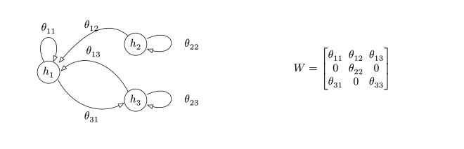
after one step of the RNN, the parameter will have influenced only . After two steps, via , it will begin to influence , and after three steps, it will have affected all the hidden units of the network. Clearly, this influence after steps will impact in a different manner for each hidden unit .
[8] introduced the Sparse n-step Approximation (SnAp-n) for the Jacobian of the network based on the previous observation. More formally, for all :
this approximation essentially defines a mask matrix (Figure 1), that will induce sparsity in the Jacobian, based on the sparsity of the network.
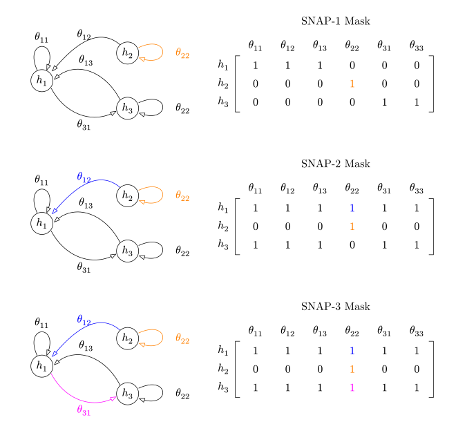
Figure 1: Masks induced by Sparse N-Step Approximation algorithm in
This -step approximation can be integrated within the algorithmic framework introduced by [5] for algorithms that approximate the in RTRL (Algorithm 1). There they define a function as a function that computes either a biased or unbiased approximation of its input and stores it in the prescribed format . We choose to work within this framework since it provides a clear description of the terms that need to be computed.
Algorithm 1: One step of approximating RTRL
Input: input , hidden state , parameters , approximation of stored in prescribed format .
Output: hidden state , approximation of in format .
Preliminary calculations
- new hidden state, based on , ,
- ,
Bring addends , in desired format
Mix two addends ,
- , where is an approximator of in format
In the case of SnAp-n:
therefore the RTRL equations can now be written as :
note that since for any , its not performing any effective masking3 on .
Since the same mask is applied at each time step, we can exploit this uniformity to optimize computational efficiency. Specifically, as highlighted by the authors of SnAp-n, it is possible to transition from the naive matrix multiplication algorithm, which operates in time (for matrices ), to an algorithm with a complexity of , where denotes the number of non-zero elements in the mask matrix . Furthermore, if the storage format is designed to leverage the sparsity of the elements involved in the computation, we can achieve significant memory savings proportional to the sparsity of the mask. In this post, we will present various algorithms designed to achieve these computational improvements. More specifically we will show how to compute , , and , with memory cost bounded by .
3 Sparse Matrices
In order to implement Algorithm 1, we have to decide on the prescribed format for storing the Jacobians. Given that we are inducing sparsity through SnAp-n, we can utilize one of the various formats developed over the past decades to represent sparse matrices. Among these, we opt to work with the Coordinate List (COO) format and the Compressed Sparse Row (CSR) format.
COO stores an array of non-zero elements and their corresponding row and column indices. In contrast, the CSR (Figure 2) format enhances memory efficiency and computational performance by storing the non-zero elements in a single array (data), along with two auxiliary arrays indicating the start of each row (indptr) and the column indices (indices) of the elements, this structure allows for faster row access operations when compared to COO.
For the purposes of implementing SnAp-n we will choose COO as the prescribed format . This choice is motivated by the following considerations.
The first one being that efficient algorithms exist to convert it to other sparse sparse formats, which might be more suitable for performing linear algebra operations. Converting from COO to CSR, when the indices are sorted lexicographically can be done by computing a prefix sum, which in turn can be performed efficiently using a parallel associative scan ([9]). This becomes important when in runtime, at every step of RTRL we have to switch to CSR for faster row access operations.
The second one is more SnAp-n specific. Suppose we can compute and (See 4, 6) in any prescribed sparse format . For the non-zero entries induced by SnAp-n in and will differ and consequently also their associated data structures, as is independent of (Recall 4). Therefore we need to devise an efficient method to add both sparse terms. When using the COO format, we have that and implementing becomes trivial. This is achieved by maintaining an array that maps each index in to its corresponding position in , so that we have:
addition of both sparse terms can now be implemented as:
This approach however requires storing an extra array, , increasing the cost for storing , but note that in general for , so its the data structures from that will dominate the memory. Also 5 is a pure function, where in addition all the array shapes involved are static and known at compile time, which will come in handy at later sections. The mixing operation can also be computed avoiding any extra storage at the expense of more operations per step, reducing significantly the time performance.
Having motivated our choice for in the following section we will present an algorithm to compute without explicitly computing the dense . To this end, we will employ a matrix coloring technique that will substantially reduce the space required for storage, as well as the computational effort needed.
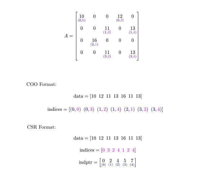
Figure 2: Matrix and its sparse representations in COO and CSR format.
4 Sparse Jacobian Computation
Let , and assume that for regardless of the input to the function, the Jacobian always keeps the following sparse structure :
Ideally we would like to take advantage of the sparsity in the Jacobian to minimize the number of evaluations required for its determination. [10] observed that a group of rows could be determined through a single evaluation, provided no two rows in the group contain a nonzero element in the same column position. Such a group of rows is defined as structurally orthogonal to each other, which differs from the common notion of orthogonality in vector spaces. A set of structurally orthogonal groups that contains all the rows of the matrix is termed a consistent partition of the matrix. A matrix clearly can be trivially partitioned into a set of structurally orthogonal groups, one group for each row, the objective therefore its to find a consistent partition with the minimum number of groups.
Define now to be a graph with vertices and edges if and only if and rows and in 6 have a nonzero in the same column position (See figure 3). If we color the graph so that no two adjacent vertices have the same color, we can obtain a consistent partition of the matrix where the groups are defined by the color of each vertex. This connection between finding consistent partition of the matrix and coloring the associated graph, was first introduced by [11].
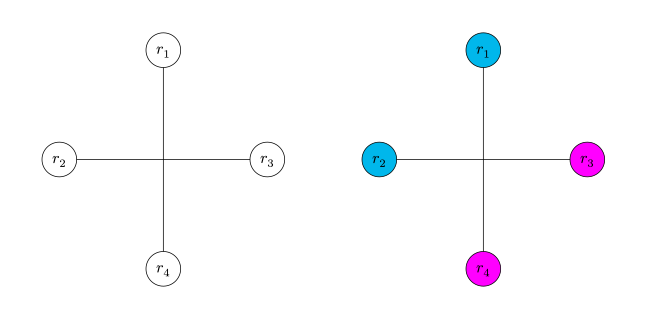
Figure 3: Induced graph and its coloring.
The resulting matrix coloring of will look like this:
Clearly we can define now and , and perform a blocked vector-Jacobian product to obtain the compressed Jacobian, from which the non zero elements of can easily be accessed and stored in :
Throughout this post we will refer to the matrix used to left multiply the Jacobian and retrieve the non-zero elements as the Jacobian projection matrix . For a detailed description of the algorithm, please refer to Algorithm 2.
Algorithm 2: Non-Zero Entries of Sparse Jacobian Using Graph Coloring.
Input: Jacobian , Sparsity Pattern .
Output: Compressed Jacobian .
- Compute the induced graph .
- Color and save the groups .
- .
- .
- For to do
- For to do
- if and only if row
- End for
- End for
In general for a function , the number of entries required to store the Jacobian is reduced by a fraction of , where is the number of colors used in the algorithm. For a standard RNN with a hidden size of , storing the dense requires memory. In contrast, for the compressed version, the memory requirement is reduced to .
While the matrix coloring algorithm enables us to uniquely determine the non-zero entries in a sparse Jacobian, a significant challenge remains: the explicit Jacobian matrix is often unavailable and computing it directly is infeasible due to its large memory requirements. To address this, we can leverage automatic differentiation tools, particularly those that implement the vector-Jacobian product (VJP) operation. These tools allow us to compute the necessary derivatives implicitly, without forming the entire Jacobian matrix.
A prominent example of such a tool is JAX [12], a high-performance library designed for numerical computing and machine learning research. JAX provides robust automatic differentiation capabilities, allowing us to compute the necessary derivatives implicitly, without forming the entire Jacobian matrix. By integrating matrix coloring with JAX's VJP functionality, we can efficiently handle sparse Jacobians, thus circumventing the substantial storage and computational costs associated with the explicit Jacobian computation.
Implementing Algorithm 2 would be straightforward if we
restricted ourselves to functions accepting a single rank-1 array, since JAX
through its jax.vjp interface combined with jax.vmap,
facilitates the computation of in a one-liner.
However, to provide a clean interface and generalize our implementation to
accommodate any RNN architecture, we must support the computation of sparse
Jacobians for functions that accept arbitrary PyTrees4. For the remainder of this
post we will refer to an arbitrary PyTree as , and to its leaves as
.
5 Sparse JACREV
Assume for simplicity that .
JAX of course allows us to compute the VJP for functions accepting an
arbitrary PyTree (Figure 4), however there is one caveat. Once
the VJP of is obtained, the cotangent vector will be applied for every
leaf in the PyTree. Since not every leaf will produce the same sparsity pattern
in the Jacobian, and therefore not the same Jacobian projection matrix ,
what we want is to compute using jax.vjp
for every leaf in without computing for ,
so that we don't waste space or perform unnecesary computations
(Figure 5).
To the best of our knowledge there is no such functionality avalaible, therefore we dig into the internals of JAX to allow such computations. Our implementation supports dense leaves and sparse leaves represented in the COO format, under the same function. Furthermore, in computing for a sparse the dimensions of the Jacobian will reflect the sparsity of the leaf, obtaining a Jacobian of dimensions . This allows us to obtain the memory gains in sparse recurrent neural networks , outlined by [8], even when there is no approximation made to the Jacobian when using the RTRL algorithm.
With the previous functionality in hand, we propose the following interface for implementing Algorithm 2:
-
def make_jacobian_projection(
    jacobian_mask: PyTree
) -> PyTree:
Must recieve a PyTree with the same structure as , where at each leaf must contain the sparsity pattern of its corresponding Jacobian. It will then compute the coloring of the induced graph for each leaf using networkx ([13]) as described in section 4, and then return the Jacobian projection matrices in a PyTree with the same structure as .
-
def sp_jacrev(
    f: Callable,
    V: PyTree,
    argnums: int | sequence[int] = 0
) -> Callable:
Mimics almost one-to-one the current
jax.jacrevthat allows the user to compute the dense jacobians, with the difference that ours allows the user to pass a PyTree with the Jacobian projection matrices to obtain the sparse Jacobians. Our implementation is fully compatible with all the JAX high level operations (jit, grad, vmap). The returned callable will compute the sparse jacobians evaluated at the primals, and return them stored in COO.
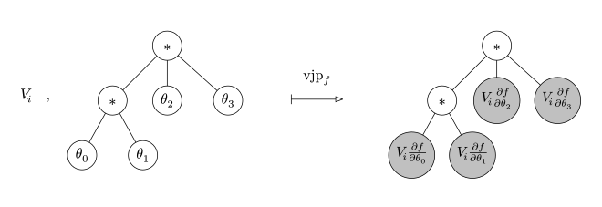
Figure 4: JAX VJP for a PyTree. Note that the contangent vector is applied for every leaf, independently if we wanted to apply it just for one leaf in specific.
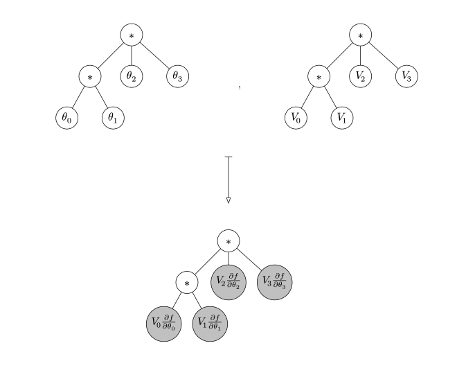
Figure 5: Custom vjp function where we accept the primal PyTree and another PyTree that contains at each leaf a differrent contangent vector that will be applied to the matching leaf in the primal PyTree.
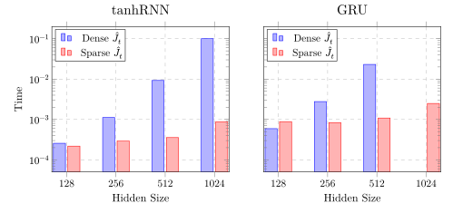
We conduct benchmarks of our implementation to measure the predicted memory savings when computing , for both a tanhRNN and standard GRU. As illustrated in Figure 6 and Figure 7, our approach demonstrates both memory and computation cost advantages when using the matrix coloring technique in comparison to the explicit computation of the Jacobian.
For profiling the memory we used pprof as recommended by the JAX developers. To ensure the correctness of our benchmarks, we provide the snapshots of the memory sate for each method where we must see a linear tree in which the root must indicate the function being used (Figure 8).
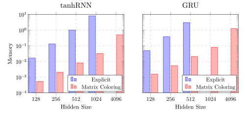
Figure 6: Memory allocated in the GPU, log scale, to compute for different architectures in a NVIDIA RTX 3090. Bars not showed indicate that we could allocate the dense Jacobians in memory. Note that it requires storage where is the numer of hidden units.
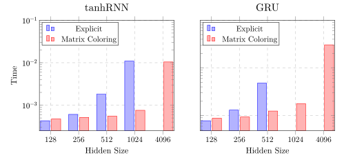
Figure 7: Time to compute for different architectures in a NVIDIA RTX 3090. Bars not showed indicate that we could allocate the dense Jacobians in memory. Note that it requires storage where is the numer of hidden units.
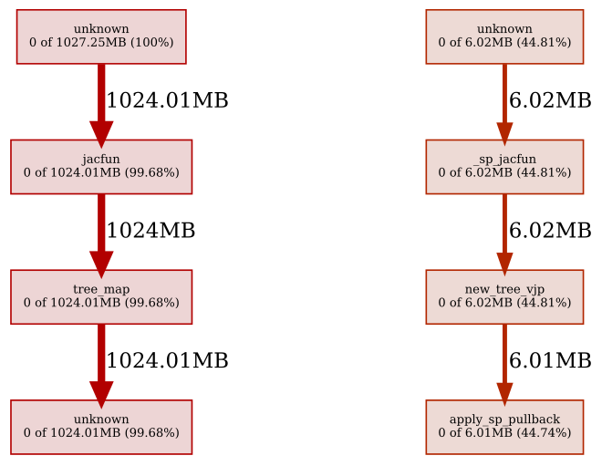
Figure 8: Flamegraph obtained by pprof of jax.jacrev and
sp_jacrev, for a tanhRNN with a hidden size of 512 units. We
omit the rest of the leafs below the last node for better visualization
purposes.
Given that we can now compute for any arbitrary recurrent neural network, , and store it in the prescribed format as defined by , in the next section we will implement a kernel to compute exploiting the sparsity of the mask involved. This will substantially reduce the computational cost, when the zero elements of the mask dominate the non-zero elements.
6 Masked Sparse Matrix Multiplication
Sparse matrix computations are crucial in scientific and engineering applications, enabling efficient handling of large-scale data. Algorithms for sparse matrix operations, such as sparse matrix-sparse matrix multiplication (SpMM) and dense-sparse matrix multiplication (DSMM) reduce memory usage and computational complexity by exploiting the sparsity of the operands.
In recent years, JAX has made significant progress enhancing its support for sparsity on GPUs by integrating with cuSPARSE, NVIDIA's library for sparse matrix operations. Despite these advancements numerous operations provided by cuSPARSE are not yet fully supported within JAX.
In this section, we introduce an algorithm to address a specific operation:
where is dense, is a sparse matrix stored in 5, and is a masking matrix also in . Since the mask matrix induces sparsity in , we aim for the resulting to be in as well. This operation is particularly relevant to us since recall that . Therefore implementing 8 efficiently will allows us to finalize the implementation of Algorithm 1 under the SnAp-n approximation.
Implementing 8 can be done in
using the most naive algorithm, where for each we perform the
dot product . This algorithm is also embarrassingly
parallelizable, excluding any parallelism within the dot product itself. To
exploit this parallelism we could use jax.vmap in combination with
JAX's support of the COO6 format.
However as we found, this approach is highly inefficient. The inefficiency
arises from accessing a column in the COO format, which is inherently slow. One
possible solution is to convert from the COO format to a CSR format, and
compute instead , as CSR allows
for efficient row access. Unfortunately, the JAX library does not support row
slicing in CSR format. We believe the reason for this limitation is that
accessing a row in CSR format does not satisfy JAX's static shape constraints.
Specifically, in CSR format, a row is accessed using
X.data[indptr[i]:indptr[i+1]], and this form of dynamic slicing is not
permitted within just-in-time compiled (JIT) functions, which is one of the
main reasons to use JAX.
Considering these constraints, we opted to implement the Masked Dense Sparse Matrix Multiplication (Masked DSMM) as a primitive operation in JAX. This implementation ensures compatibility with JIT compiled functions. The primitive operates on CSR sparse matrices, and the algorithm is detailed in Algorithm 3.
Algorithm 3: Masked Sparse-Matrix Dense-Matrix Multiplication
Input: Mask , , .
Output: .
- Procedure Masked-SpMM(, , )
- For all to do in parallel
- If then
- Else
- End if
- End for
- End procedure
For the CPU support we implemented the primitive in NUMBA ([14]) and
take advantage of their cfunc decorator that creates a compiled
function callable from foreign C code. We then take the address of this JITed
function and register it in the XLA compiler through their custom call API. For
the GPU support the process becomes more intricate and requires knowledge of
Python and C programming. The steps required to add a custom GPU primitive in
JAX can be seen in Figure 9.
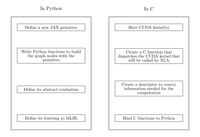
Figure 9: Steps required to add a new CUDA primitive to JAX.
Before delving into CUDA programming, it is prudent to check whether existing libraries already implement the desired kernel. To the best of our knowledge, the primitive described in equation 8 is absent in current GPU Sparse General Matrix Multiplication (SpGEMM) libraries. We identified only two relevant libraries: GraphBlast ([15]) and cuSPARSE.
GraphBlast implements the GraphBlas API specification ([16]), which stipulates that a compliant library should include the primitive in 8. However, an examination of GraphBlast's source code reveals that it does not support masking when one of the operands is dense, as required for our application. Although we could convert our first operand to a sparse format to use their implementation, this approach is infeasible. For our use case represents , which can indeed be sparse and constant. However, outside the regime of a Linear RNN, the sparsity of the dynamics Jacobian varies depending on the input. This variability violates JAX's static shape constraints when constructing a COO or CSR matrix, as the number of non-zero entries must be static and known at compile time.
On the other hand, cuSPARSE offers the function cusparseSDDMM for
masking the output, which only works with dense inputs to produce a sparse
output. For RNNs trained with Real-Time Recurrent Learning (RTRL), reverting to
a dense representation of the Jacobians is prohibitive, as discussed in the
previous section. This limitation in existing libraries motivated us to create
our own custom kernels, specifically tailored to address the requirements of
our Masked Dense Sparse Matrix Multiplication (Masked DSMM) operations.
To invoke a CUDA kernel, we must specify the grid size and block dimensions. Since Algorithm 3 parallelizes over the non-zero elements of the mask we opted for a one-dimensional grid where the grid size is determined by . Here indicates the number of threads per block, which we set to be 1024.
With the Masked DSMM primitive established, we can now fully implement Algorithm 1. Figure 10 showcases benchmarks of our implementation, contrasting it with the original code provided by [8] for SnAp-1. Our implementation demonstrates an order of magnitude increase in speed compared to the original code, thereby validating the optimizations developed throughout this post. Specifically, our implementation aligns more closely with the theoretical improvements outlined in their publication, particularly when comparing SnAp-1 with Backpropagation Through Time (BPTT) for hidden sizes less than 512. Figure 11 reports the time required to compute the gradients for a full sequence of input-output pairs, rather than just a single step.
Figure 10: Time to compute one step of SnAp-1 for different architectures in a NVIDIA RTX 3090.
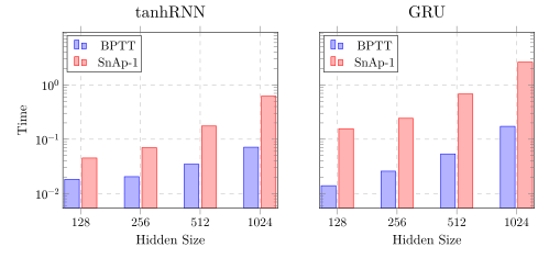
Figure 11: Time to compute for BPTT and SnAp-1 in a NVIDIA RTX 3090.
For highly sparse networks where SnAp-2 and SnAp-3 are applicable, we are unable to provide benchmarks as the corresponding code was not released. However during the development of the library we observed that the performance of our Masked DSMM diminishes as the density7 of the Jacobian falls below 0.01. Dense Matrix Multiplications are highly optimized operations that exploit memory coalescence, with cache timing being a critical factor at this level of parallelism. Our implementation achieves good memory coalescence when accessing rows of the sparse matrix. However, accessing columns results in numerous cache misses due to non-contiguous memory access patterns. This is a big limitation of our kernel, but we believe there is a lot of improvement can be made, since we just implemented the most naive algorithm we could think of. There is an existing line of research that attempts to improve the memory coalescence when using sparse operands, we refer the interested reader to [17], [18], [19], [20] among others.
We conclude this post by noting that the source code for all discussed algorithms is available as an open-source package in snapjax. In addition to the SnAp-N approximations we implement the exact RTRL algorithm for any class of single-layer RNNs. For general multilayer RNNs we implement the approximation rule introduced in [21], and if we restrict to layers following:
we implement the exact RTRL gradient computations.
References
Notes
-
A derivation for RNNs and a discussion of online parameter updates appear in Real-Time Recurrent Learning: Training Dynamics. ↩
-
BPTT uses vector–Jacobian products and reverse-mode differentiation instead of storing the full state–parameter Jacobian. Its parameter-gradient storage is , but conventional full-sequence BPTT also stores forward activations, so its total memory use grows with sequence length. ↩
-
This only holds for RNNs in which a parameter only affects one hidden unit in one time step as noted by the authors. ↩
-
A PyTree is (Verbatim from [22]) any arbitrarily nested composition of ‘node’ types (dictionaries, lists, and tuples) containing ‘leaf’ types (all other Python types as well as Rank-N Arrays). ↩
-
JAX actually prioritizes support for BCOO (Batch COO) and BCSR (Batch CSR). We work with these formats but in the text we just name then COO and CSR respectively. ↩
-
Density is defined as , where is the level of sparsity. ↩